December 2013

2013: Lessons Learned and Revisiting Some Studies

The year is over in a few hours and I thought it would be nice to do a quick review of the year, revisit some studies and the most popular posts of the year, as well as share some thoughts on my performance in 2013 and my goals for 2014.

Revisiting Old Studies

IBS

IBS did pretty badly in 2012, and didn’t manage to reach the amazing performance of 2007-2010 this year either. However, it still worked reasonably well: IBS < 0.5 led to far higher returns than IBS > 0.5, and the highest quarter had negative returns. It still works amazingly well as a filter. Most importantly the magnitude of the effect has diminished. This is partly due to the low volatility we’ve seen this year. After all IBS does best when movements are large, and SPY’s 10-day realized volatility never even broke 20% this year. Here are the stats:

UDIDSRI

The original post can be found here. Performance in 2013 hasn’t been as good as in the past, but was still reasonably OK. I think the results are, again, at least partially due to the low volatility environment in equities this year.

UDIDSRI performance, close-to-close returns after a zero reading.

DOTM seasonality

I’ve done 3 posts on day of the month seasonality (US, EU, Asia), and on average the DOTM effect did its job this year. There are some cases where the top quarter does not have the top returns, but a single year is a relatively small sample so I doubt this has any long-term implications. Here are the stats for 9 major indices:

Day of the month seasonality in 2013

VIX:VXV Ratio

My studies on the implied volatility indices ratio turned out to work pretty badly. Returns when the VIX:VXV ratio was 5% above the 10-day SMA were -0.03%. There were no 200-day highs in the ratio in 2013!

Performance

Overall I would say it was a mixed bag for me this year. Returns were reasonably good, but a bit below my long-term expectations. It was a very good year for equities, and my results can’t compete with SPY’s 5.12 MAR ratio, which makes me feel pretty bad. Of course I understand that years like this one don’t represent the long-term, but it’s annoying to get beaten by b&h nonetheless.

Some strategies did really well:

Others did really poorly:

The Good

Risk was kept under control and entirely within my target range, both in terms of volatility and maximum drawdown. Even when I was at the year’s maximum drawdown I felt comfortable…there is still “psychological room” for more leverage. Daily returns were positively skewed. My biggest success was diversifying across strategies and asset classes. A year ago I was trading few instruments (almost exclusively US equity ETFs) with a limited number of strategies. Combine that with a pretty heavy equity tilt in the GTAA allocation, and my portfolio returns were moving almost in lockstep with the indices (there were very few shorting opportunities in this year’s environment, so the choice was almost always between being long or in cash). Widening my asset universe combined with research into new strategies made a gigantic difference:

The Bad

I made a series of mistakes that significantly hurt my performance figures this year. Small mistakes pile on top of each other and in the end have a pretty large effect. All in all I lost several hundred bp on these screw-ups. Hopefully you can learn from my errors:

Back in March I forgot the US daylight savings time kicks in earlier than it does here in Europe. I had positions to exit at the open and I got there 45 minutes late. Naturally the market had moved against me.
A bug in my software led to incorrectly handling dividends, which led to signals being calculated using incorrect prices, which led to a long position when I should have taken a short. Taught me the importance of testing with extreme caution.
Problems with reporting trade executions at an exchange led to an error where I sent the same order twice and it took me a few minutes to close out the position I had inadvertently created.
I took delivery on some FX futures when I didn’t want to, cost me commissions and spread to unwind the position.
Order entry, sent a buy order when I was trying to sell. Caught it immediately so the cost was only commissions + spread.
And of course the biggest one: not following my systems to the letter. A combination of fear, cowardice, over-confidence in my discretion, and under-confidence in my modeling skills led to some instances where I didn’t take trades that I should have. This is the most shameful mistake of all because of its banality. I don’t plan on repeating it in 2014.

Goals for 2014

Beat my 2013 risk-adjusted returns.
Don’t repeat any mistakes.
Make new mistakes! But minimize their impact. Every error is a valuable learning experience.
Continue on the same path in terms of research.
Minimize model implementation risk through better unit testing.

Most Popular

Finally, the most popular posts of the year:

The original IBS post. Read the paper instead.
Doing the Jaffray Woodriff Thing. I still need to follow up on that…
Mining for Three Day Candlestick Patterns, which also spawned a short series of posts.

I want to wish you all a happy and profitable 2014!

annual review, IBS effect, seasonality, UDIDSRI, VIX, VXV

Reverse Engineering DynamicHedge’s Alpha Curves, Part 1 of 3: Dynamic Time Warping

DynamicHedge recently introduced a new service called “alpha curves”: the main idea is to find patterns in returns after certain events, and present the most frequently occurring patterns. In their own words, alpha curves “represent a special blend of uniqueness and repeatability”. Here’s what they look like, ranked in order of “pattern dominance”. According to them, they “use different factors other than just returns”. We can speculate about what other factors go into it, possibly something like maximum extension or the timing of maxima and minima, but I’ll keep it simple and only use returns.

In this post I’ll do a short presentation of dynamic time warping, a method of measuring the similarity between time series. In part 2 we will look at a clustering method called K-medoids. Finally in part 3 we will put the two together and generate charts similar to the alpha curves. The terminology might be a bit intimidating, but the ideas are fundamentally highly intuitive. As long as you can grasp the concepts, the implementation details are easy to figure out.

To be honest I’m not so sure about the practical value of this concept, and I have no clue how to quantify its performance. Still, it’s an interesting idea and the concepts that go into it are useful in other areas as well, so this is not an entirely pointless endeavor. My backtesting platform still can’t handle intraday data properly, so I’ll be using daily bars instead, but the ideas are the same no matter the frequency.

So, let’s begin with why we need DTW at all in the first place. What can it do that other measures of similarity, such as Euclidean distance and correlation can not? Starting with correlation: one must keep in mind that it is a measure of similarity based on the difference between means. Significantly different means can lead to high correlation, yet strikingly different price series. For example, the returns of these two series have a correlation of 0.81, despite being quite dissimilar.

A second issue, comes up in the case of slightly out of phase series, which are very similar but can have low correlations and high Euclidean distances. The returns of these two curves have a correlation of .14:

So, what is the solution to these issues? Dynamic Time Warping. The main idea behind DTW is to “warp” the time series so that the distance measurement between each point does not necessarily require both points to have the same x-axis value. Instead, the points further away can be selected, so as to minimize the total distance between the series. The algorithm (the original 1987 paper by Sakoe & Chiba can be found here) restricts the first and last points to be the beginning and end of each series. From there, the matching of points can be visualized as a path on an n by m grid, where n and m are the number of points in each time series.

Source: Elena Tsiporkova, Dynamic Time Warping Algorithm for Gene Expression Time Series

The algorithm finds the path through this grid that minimizes the total distance. The function that measures the distance between each set of points can be anything we want. To restrict the number of possible paths, we restrict the possible points that can be connected, by requiring the path to be monotonically increasing, limiting the slope, and restricting how far away from a straight line the path can stray. The difference between standard Euclidean distance and DTW can be demonstrated graphically. In this case I use two sin curves. The gray lines between the series show which points the distance measurements are done between.

DTW

Euclidean

Notice the warping at the start and end of the series, and how the points in the middle have identical y-values, thus minimizing the total distance.

What are the practical applications of DTW in trading? As we’ll see in the next parts, it can be used to cluster time series. It can also be used to average time series, with the DBA algorithm. Another potential use is k-nn pattern matching strategies, which I have experimented with a bit…some quick tests showed small but persistent improvements in performance over Euclidean distance.

If you want to test it out yourselves, there are plenty of tools out there. I’m using the NDTW .NET library. There are libraries available for R and python as well.

alpha curves, DTW, Dynamic Time Warping

The QUSMA Data Management System Is Now Open Source

The QUSMA Data Management System (QDMS) is an application for acquiring, managing, and distributing low-frequency historical and real-time data, written in C#.

QDMS uses a client/server model. The server acts as a broker between clients and external data sources. It also manages metadata on instruments, and local storage of historical data. Finally it also functions as a UI for managing the metadata & data, as well as importing/exporting data from and to CSV files.

Currently it supports two external data sources: Interactive Brokers and Yahoo, but I’ll be adding more in the future.

Note that it’s not “production-ready” right now. There are still a few bugs to iron out, and it also uses unstable 3rd party libraries (the alpha version of the MySQL .NET connector, because it’s the only one that supports Entity Framework 6). All the “core” functionality is implemented and functional, however.

You can find the code here: https://github.com/qusma/qdms. I’m releasing it under the permissive BSD License. Contributions by way of pull requests are more than welcome. If you’d like to make any feature requests or just flame me for the quality of my code, leave a comment right here.

I personally use it in my backtester and portfolio performance evaluation applications, and I’m in the process of integrating it with my live trading app as well.

Using the client is easy, let’s take a look at some code examples:

Getting a list of all instruments:

List<Instrument> instruments = client.FindInstruments();

Searching for a specific instrument, for example SPY:

Instrument spy = client.FindInstruments(new Instrument { Symbol = "SPY" }).FirstOrDefault();

Requesting historical data:

var histRequest = new HistoricalDataRequest(
                    spy,
                    BarSize.OneDay,
                    new DateTime(2013, 1, 1),
                    new DateTime(2013, 1, 15));

client.RequestHistoricalData(histRequest);

Requesting real time data:

var rtRequest = new RealTimeDataRequest(spy, BarSize.OneSecond);
client.RequestRealTimeData(rtRequest);

Some screenshots:

Instrument metadata.

Adding a new instrument from Interactive Brokers.

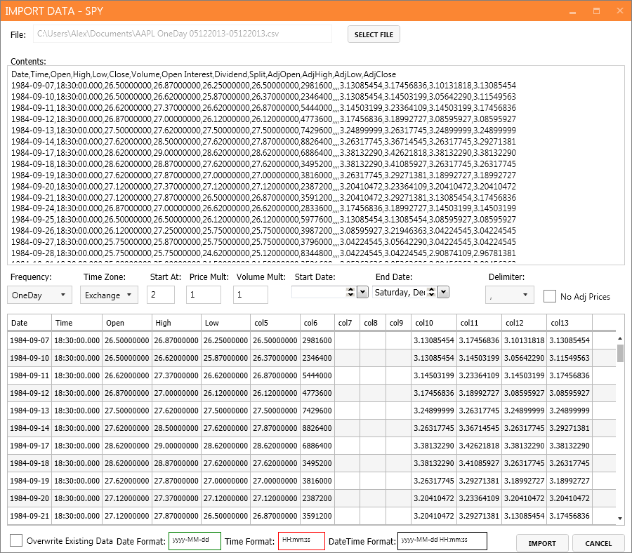
Importing data from a CSV file.

Main server screen.

C#, QDMS

Equity Returns Following Extreme VIX and WVF Movements, Part 2

Part 1 covered the relation between VIX/WVF extreme movements and SPY; here we take a wider look, covering a large number of international equity ETFs.

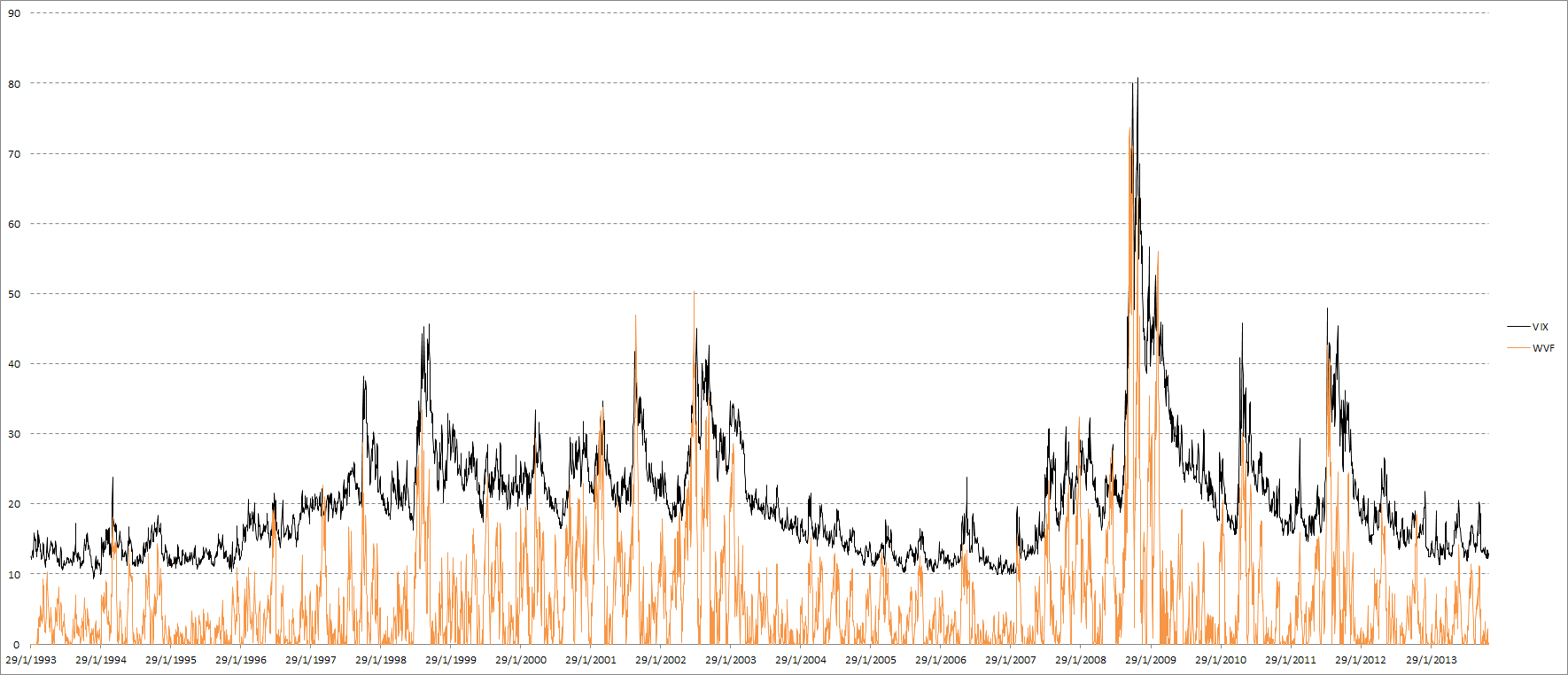
The main idea behind WVF is that it acts similarly to VIX in high-volatility situations, possibly enough to serve as an implied volatility substitute in cases where such an index does not exist. It can be useful to “confirm” signals based on implied volatility, or to replace them completely in cases where no implied volatility index exists. First of all let’s take a look at an updated VIX & SPY WVF chart:

VIX & SPY WVF

The first post was a while ago, so let’s check how VIX and WVF have performed for SPY since then. The number of signals is very small, and WVF alone has underperformed compared to its historical results, but once again we see that the combination of VIX and WVF offered by far the best results:

Signal results on SPY since 25 Oct. 2012

Let’s take a look at how these signals work internationally:

Close-to-close returns following 100-day 99th percentile VIX return.

It’s clear that using only VIX is pretty useless. Overall the returns are not significantly different from zero, and are even negative in many cases. Let’s check out WVF, which appears to work far better across most ETFs:

Close-to-close returns following 100-day 99th percentile WVF change.

Finally, when VIX and WVF extreme movements coincide, the results look fantastic:

Simultaneous VIX and WVF extreme movements.

Note that even in cases where WVF alone did not show good results (the VT and WVF ETFs for example), combining VIX and WVF still results in great improvement. There is an important, general lesson here about using non-price data as trade set-ups. With few exceptions, implied volatility, breadth, seasonality, etc. need to be “confirmed” by price to actually be useful.

VIX, WVF

Month: December 2013